Mortgage Stress Tests for Analysts: Compare Countries, Not Loans
2026-10-14

Mortgage portfolio stress testing simulates portfolio-level losses under adverse but plausible macro-financial scenarios to quantify tail risk and inform capital and macroprudential policy. The goal is to learn how a book of home loans would hold up if house prices, rates and employment turned against it. The BIS, the IMF and the EBA set the standards analysts work from, and each is covered below.
TL;DR:
- Models that link loan performance to macroeconomic drivers can better handle crisis shifts than standard empirical models; integrated tests capture risk interactions.
- Anchor adverse scenarios in defensible tail estimates, keep house prices, rates, and unemployment paths internally consistent, and use reverse tests to identify capital breaking points.
- Group loan level data by vintage, LTV, and LTI; check that simulation results stabilize as draws increase before relying on tail loss percentiles.
- EBA reporting constraints include static balance sheets, no cures for Stage 3 exposures, and risk exposure amount floors, so results are not forecasts.
- Capital buffers and Pillar 2 add ons target existing loans, while LTV and LTI caps mainly shape new lending; supervisors retain judgment.
Table of Contents
- What a mortgage portfolio stress test measures
- Which modeling approach fits your portfolio?
- How do you design and calibrate the adverse scenario?
- What data and simulation setup do you need?
- How do you turn stress results into policy action?
- A practitioner checklist for a credible program
- Where did mortgage stress testing come from?
- Where do portfolio stress test results get used?
- What are the limits of portfolio stress testing?
- Why consistent official data matters for cross-country work
- Where to find calibration data on Fiatmap
- FAQ
- Sources
What a mortgage portfolio stress test measures
This article covers the portfolio-level definition only: a simulation of an entire loan book, run by a bank or supervisor to see aggregate losses. It is not a check of whether any single household could keep paying. Practitioners draw the same line: portfolio tests simulate an entire cycle with Monte Carlo or semi-structural methods to estimate an aggregate loss distribution for systemic shocks.
Typical outputs are point-in-time probabilities of default (PD), loss given default (LGD) by loan bucket, and portfolio loss metrics such as value at risk and tail percentiles. The horizon depends on the exercise, since house-price corrections and unemployment shocks can take time to affect defaults.
The scenario itself needs discipline. The BIS describes an adverse scenario as conditions significantly more negative than baseline, covering material risks, internally consistent across key variables, and documented wherever a material risk is excluded.
Which modeling approach fits your portfolio?
Several modeling approaches are used. Pick based on how much history you trust and how many risks you need to correlate.
- Semi-structural models simulate PD and LGD as functions of macro drivers and the loan life cycle. IMF researchers favor them because standard empirical models often fail in crises when structural shifts break historical relationships.
- Monte Carlo and non-parametric resampling build an empirical loss distribution from observed outcomes, which also lets you test whether regulatory coverage holds up under stress, as in this BIS workshop paper.
- Integrated versus piecewise designs differ in scope. Piecewise tests stress one factor at a time. Integrated designs let market, credit and liquidity risks interact, which matters because correlations rise in severe shocks, as this BIS survey of methodologies explains.
Semi-structural models also support counterfactuals, such as asking what a lower LTV cap would have done to losses. That is why we see them used for calibrating borrower-based tools.
Pro Tip: Run every key parameter across a sensitivity range rather than a point estimate, since estimation uncertainty can move tail losses more than the scenario itself.
How do you design and calibrate the adverse scenario?
Severity needs a defensible anchor. IMF research recommends Growth-at-Risk and House-price-at-Risk approaches to inform tail-risk scenarios and to benchmark projected losses against crisis-era loss metrics, so you can gauge net systemic risk rather than a raw number.
Paths for interest rates, unemployment and house prices must move together over the horizon. A price collapse with falling unemployment is not a scenario, it is a contradiction. Our mortgage rate glossary is a useful reference when building the rate leg.
Reverse stress testing works backward: find the combination of shocks that breaches a capital or solvency threshold, then judge how plausible it is.
- Pull the national house-price and credit history and fit tail estimates.
- Set the headline shock at a tail percentile you can justify.
- Build rate and unemployment paths consistent with that shock.
- Run a reverse test to locate the breaking point.
- Document every assumption and each excluded risk.
What data and simulation setup do you need?
The minimum loan-level fields are origination vintage, outstanding balance, LTV, LTI or DTI, tenor and collateral quality. Our loan-to-value guide shows how LTV buckets are built.
- Bucketing: group loans by vintage, LTV and LTI. Vintage matters because it fixes when rates reprice and how much tenor remains.
- Simulation design: the IMF’s semi-structural model works on bank portfolio data split by vintage, LTI and LTV, simulates PD and LGD with repeated draws (its example settings are N=2000 and K=10,000), then aggregates bucket outputs into portfolio PD, LGD and loss rate.
- Reporting: the EBA methodological note fixes constrained templates, static balance-sheet assumptions, no cures for Stage 3 exposures and risk-exposure-amount floors. Its template guidance also requires restating starting points under CRR3.
- Convergence: check that results stabilize as draws increase before you trust a tail percentile.
How do you turn stress results into policy action?
Benchmark stressed losses against historical crisis loss rates and against regulatory hurdle metrics. A figure means little until it sits beside a real downturn and a capital buffer.
Policy levers then split by target. The countercyclical capital buffer (CCyB) and Pillar 2 add-ons act on the capital held against existing stock. Borrower-based caps on LTV and LTI mostly shape new lending. IMF analysis of Spain finds collateral-based measures like LTV caps can sharply reduce portfolio losses under adverse conditions, and notes that Switzerland’s FINMA imposed 15 Pillar 2 capital add-ons at the end of 2024 where mortgage stress tests showed buffers could not absorb projected losses. The IMF’s Swiss assessment adds that loan-by-loan reporting will expand from 2027.

Tests inform decisions. They do not automatically trigger one prescribed outcome, and supervisors weigh the findings alongside judgment.
A practitioner checklist for a credible program
- Governance: board sign-off, named model owners, written documentation.
- Validation: backtesting, sensitivity bands, and tests of stress severity.
- Concentration: BIS material stresses that concentration risk cannot be modeled in isolation, so use multi-factor models with correlations estimated endogenously where possible. Factor-concentration tests that truncate systematic factors are described in this BIS paper.
- Operations: assume realistic collections capacity, mortgage insurance payouts and the cost of handling elevated delinquencies.
Pro Tip: Stress your operational assumptions too: a collections team sized for normal arrears can fail long before capital does.
Where did mortgage stress testing come from?
Early macro stress testing was a supervisory experiment. By the early 2000s, BIS surveys were codifying stages: scope, scenario calibration, then quantifying balance-sheet effects through financial soundness indicators or integrated loss distributions. Housing was an obvious target.
APRA’s 2003 exercise became a reference case. Its regulatory case study mapped a 30% house-price fall into higher PDs and LGDs, lower mortgage insurance recoveries and extra resolution costs, and produced industry-level solvency findings followed by supervisory action. APRA later summarized the lesson that a successful test is an end-to-end process: design, granular implementation, follow-up and public communication.
Regulation then moved from ad hoc tests to standing frameworks. BIS guidance now treats stress testing as part of governance, covering material risks, reverse tests, and use in capital planning and macroprudential calibration. In Europe, the EBA runs EU-wide exercises whose comparable results feed supervisory dialogue, and the 2027 draft templates demand granular projections by country, scenario and portfolio.

Where do portfolio stress test results get used?
The same simulation serves several audiences. Supervisors use it to compare banks and set add-ons, as in the Swiss case above. Central banks and finance ministries use it to calibrate borrower-based caps before introducing them. Bank risk teams use it for capital planning and for deciding where to tighten underwriting.
Household-sector work shows a further use. IMF assessments of the Netherlands combined loan-level PD estimation, general equilibrium models for macro effects, and sensitivity and concentration analysis to identify vulnerable household segments: young, low-income and high-LTV or high-LTI borrowers. That tells a policymaker where a cap bites.
For investors and cross-country analysts, results translate into comparative judgment: which markets carry thin buffers against price falls, and which have levers ready. Price dispersion matters here, and our story on the same mortgage priced very differently shows how far rate environments diverge. Partner guidance on stress-test rules for first-time buyers illustrates how one jurisdiction applies borrower-based rules, which is a useful contrast with portfolio tests.
What are the limits of portfolio stress testing?
Every test inherits the weaknesses of its inputs. Historical relationships break in crises, which is the very reason semi-structural models exist, yet those models rest on assumptions about the loan life cycle that can also be wrong. Parameter uncertainty can swamp scenario differences, so a single headline loss figure overstates precision.
Scenario design carries judgment. Choosing a tail percentile is defensible but never objective, and an exclusion of a material risk can quietly shrink results. Supervisory constraints help comparability but limit realism: static balance sheets, floors and no cures for Stage 3 exposures mean reported numbers are not forecasts.
Data is the practical bottleneck. Loan-level fields are often incomplete for older vintages, and cross-country comparison suffers when definitions of LTV, income or default differ. Concentration and correlation are hard to estimate, and treating them separately understates tail risk. Finally, endogenous behavior, such as lenders tightening credit or borrowers defaulting strategically once prices fall, is difficult to capture, so results are best read as a disciplined range, not a prediction.
Why consistent official data matters for cross-country work
Calibrating Growth-at-Risk or House-price-at-Risk across countries only works when inputs share definitions. We draw our data exclusively from official statistics. This includes mortgage rates, house-price growth and macro series from different markets. Without that, a cross-country gap in tail severity may just reflect a difference in how each country measures prices. The lesson is simple: fix the data first, then argue about the model.
— Torstein
Where to find calibration data on Fiatmap
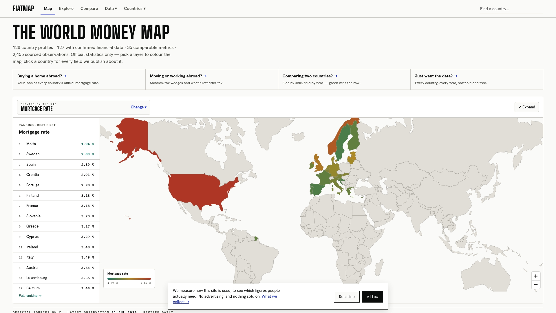
Assembling consistent inputs is usually the slowest part of building a cross-country scenario, and we built our tools to shorten it. Our Global Money Dataset is free, uses official sources only, and downloads in CSV and JSON for direct use in your calibration.
- Mortgage rates by country for the interest-rate leg of a scenario
- House price growth map to inform country-level HaR calibration
- Mortgage amortization explained for outstanding exposure over the stress horizon
- Downloadable country datasets for GaR and scenario building
Start with the dataset, pull your countries, and build your first scenario path today.
FAQ
What is a mortgage stress test at portfolio level?
It is a simulation of losses across a whole mortgage book under an adverse macro scenario. It produces portfolio PD, LGD and loss rate to show how much capital a shock could consume. It is distinct from checking whether one borrower can afford payments.
How long is the typical stress test horizon?
Most exercises run two to three years, long enough for house-price falls and unemployment to feed through into defaults. The EBA’s 2025 methodological note sets the scope and constraints for its exercise.
What is the difference between PD and LGD in a stress test?
PD is the probability that a loan defaults, and LGD is the share of exposure lost once it does. Stress tests raise both under the adverse scenario, since falling collateral values increase LGD while unemployment and rate increases raise PD.
Do stress test results force a specific policy response?
No. Results inform decisions on capital buffers, Pillar 2 add-ons or borrower-based caps, but supervisors weigh them with judgment. A weak result may lead to an add-on in one country and a lending cap in another.
Sources
- Bis
- Stress Testing and Calibration of Macroprudential Policy Tools, WP/20/165, August 2020
- Stress Testing and Calibration of Macroprudential Policy Tools* in: IMF Working Papers Volume 2020 Issue 165 (2020)
- 2025 EU-WIDE STRESS TEST
Recommended
The figures on this site are collected from official statistics and each carries its own source and date — see /sources and the dataset. Where this article states a number, the country and ranking pages are what it should agree with.